---
title: "Part 3: Geological Controls & Domain Definition"
subtitle: "Connecting Numbers to Rocks - The Path to Robust Estimation Domains"
author: "Ghozian Islam Karami"
date: "2025-10-05"
categories: [EDA, Geological Domains, Domaining, Resource Estimation]
image: "Part3.png"
format:
html:
code-fold: true
code-tools: true
toc: true
toc-depth: 3
---
## Introduction
We've validated our data ([Part 1](../Data Validation/)), explored spatial patterns, and characterized statistical distributions ([Part 2](../Spatial Statistics/)). Now comes the most critical step: **connecting numbers to geology**.
**Pillar 4: Geological Controls Analysis** transforms statistical insights into geologically defensible estimation domains - the backbone of reliable resource models.
## The Critical Question
> **"Where is mineralization located and WHY?"**
This isn't just about mapping high grades. It's about understanding the **geological controls** that govern mineralization:
- Which rock types host mineralization?
- Are there geochemical relationships between elements?
- How does grade behave at geological contacts?
- What structural controls exist?
::: {.callout-important}
## Why Geological Domains Matter
Poor domaining is a leading cause of resource estimation failure:
- Mixed populations create unrealistic variograms
- Inappropriate kriging produces smoothing artifacts
- Classification confidence is compromised
- Mining selectively targets become unrealistic
**Good domains = Reliable estimates**
:::
## Setup
```{r}
#| message: false
#| warning: false
library(dplyr)
library(tidyr)
library(ggplot2)
library(plotly)
library(DT)
library(RColorBrewer)
library(GGally)
library(patchwork)

# Create simulated drilling data with geological controls
set.seed(456)
n_holes <- 50

collar <- data.frame(
  hole_id = paste0("DDH", sprintf("%03d", 1:n_holes)),
  x = runif(n_holes, 500000, 501000),
  y = runif(n_holes, 9000000, 9001000),
  rl = runif(n_holes, 100, 200)
)

# Generate assay data with lithology-controlled grades
litho_codes <- c("Andesite", "Diorite", "Mineralized_Zone", "Altered_Volcanics")
litho_grade_means <- c(0.5, 0.8, 3.5, 2.0)  # Different grades by lithology

assay_list <- lapply(1:n_holes, function(i) {
  n_intervals <- sample(15:25, 1)
  depths <- seq(0, by = 2, length.out = n_intervals)

  # Assign lithology to each interval
  litho_idx <- sample(1:length(litho_codes), n_intervals - 1, replace = TRUE,
                     prob = c(0.3, 0.2, 0.3, 0.2))

  # Generate grades based on lithology
  au_grades <- sapply(litho_idx, function(idx) {
    max(0, rnorm(1, mean = litho_grade_means[idx], sd = 1.5))
  })

  # Correlated Ag and Cu
  ag_grades <- au_grades * runif(n_intervals - 1, 8, 12) + rnorm(n_intervals - 1, 0, 5)
  cu_grades <- au_grades * 0.3 + rnorm(n_intervals - 1, 0, 0.3)

  data.frame(
    hole_id = collar$hole_id[i],
    from = depths[-length(depths)],
    to = depths[-1],
    au_ppm = pmax(0, au_grades),
    ag_ppm = pmax(0, ag_grades),
    cu_pct = pmax(0, cu_grades),
    lithology = litho_codes[litho_idx]
  )
})

combined_data <- do.call(rbind, assay_list) %>%
  left_join(collar, by = "hole_id") %>%
  janitor::clean_names()

# Prepare standard formats
collar_std <- collar %>% janitor::clean_names()
assay_std <- combined_data %>% select(hole_id, from, to, au_ppm, ag_ppm, cu_pct)
lithology_std <- combined_data %>% select(hole_id, from, to, lithology)
```
---
# PILLAR 4: Geological Controls Analysis
## Part A: Lithology Analysis
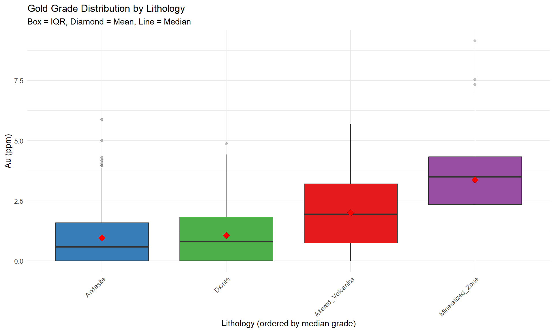
### Grade Distribution by Rock Type
The most fundamental control: **which rocks contain ore?**
```{r}
#| fig-width: 10
#| fig-height: 6
#| warning: false
# Calculate statistics by lithology
litho_summary <- combined_data %>%
  group_by(lithology) %>%
  summarise(
    n = n(),
    mean_au = mean(au_ppm, na.rm = TRUE),
    median_au = median(au_ppm, na.rm = TRUE),
    max_au = max(au_ppm, na.rm = TRUE),
    sd_au = sd(au_ppm, na.rm = TRUE)
  ) %>%
  arrange(desc(mean_au))

# Create color palette
n_litho <- length(unique(combined_data$lithology))
litho_colors <- setNames(
  brewer.pal(max(3, min(n_litho, 9)), "Set1")[1:n_litho],
  sort(unique(combined_data$lithology))
)

# Boxplot with statistical annotations
p_litho_box <- ggplot(combined_data, aes(x = reorder(lithology, au_ppm, FUN = median),
                                          y = au_ppm,
                                          fill = lithology)) +
  geom_boxplot(outlier.alpha = 0.3) +
  stat_summary(fun = mean, geom = "point", shape = 23, size = 3,
               fill = "red", color = "darkred") +
  scale_fill_manual(values = litho_colors) +
  labs(
    title = "Gold Grade Distribution by Lithology",
    subtitle = "Box = IQR, Diamond = Mean, Line = Median",
    x = "Lithology (ordered by median grade)",
    y = "Au (ppm)"
  ) +
  theme_minimal() +
  theme(
    axis.text.x = element_text(angle = 45, hjust = 1),
    legend.position = "none"
  )

p_litho_box
```
### Statistical Summary by Lithology
```{r}
datatable(litho_summary,
          caption = "Table 1: Gold Statistics by Lithology",
          options = list(pageLength = 10)) %>%
  formatRound(columns = c('mean_au', 'median_au', 'max_au', 'sd_au'), digits = 3) %>%
  formatStyle(
    'mean_au',
    background = styleColorBar(litho_summary$mean_au, 'lightblue'),
    backgroundSize = '100% 90%',
    backgroundRepeat = 'no-repeat',
    backgroundPosition = 'center'
  )
```
::: {.callout-note}
## Geological Interpretation
From this analysis, identify:
- **Primary ore hosts**: Lithologies with highest mean/median grades
- **Barren waste**: Low-grade lithologies to exclude
- **Grade variance**: High CV suggests mixed mineralization styles
- **Outlier behavior**: Which rocks have extreme values?
**Action**: Candidate lithologies for separate estimation domains
:::
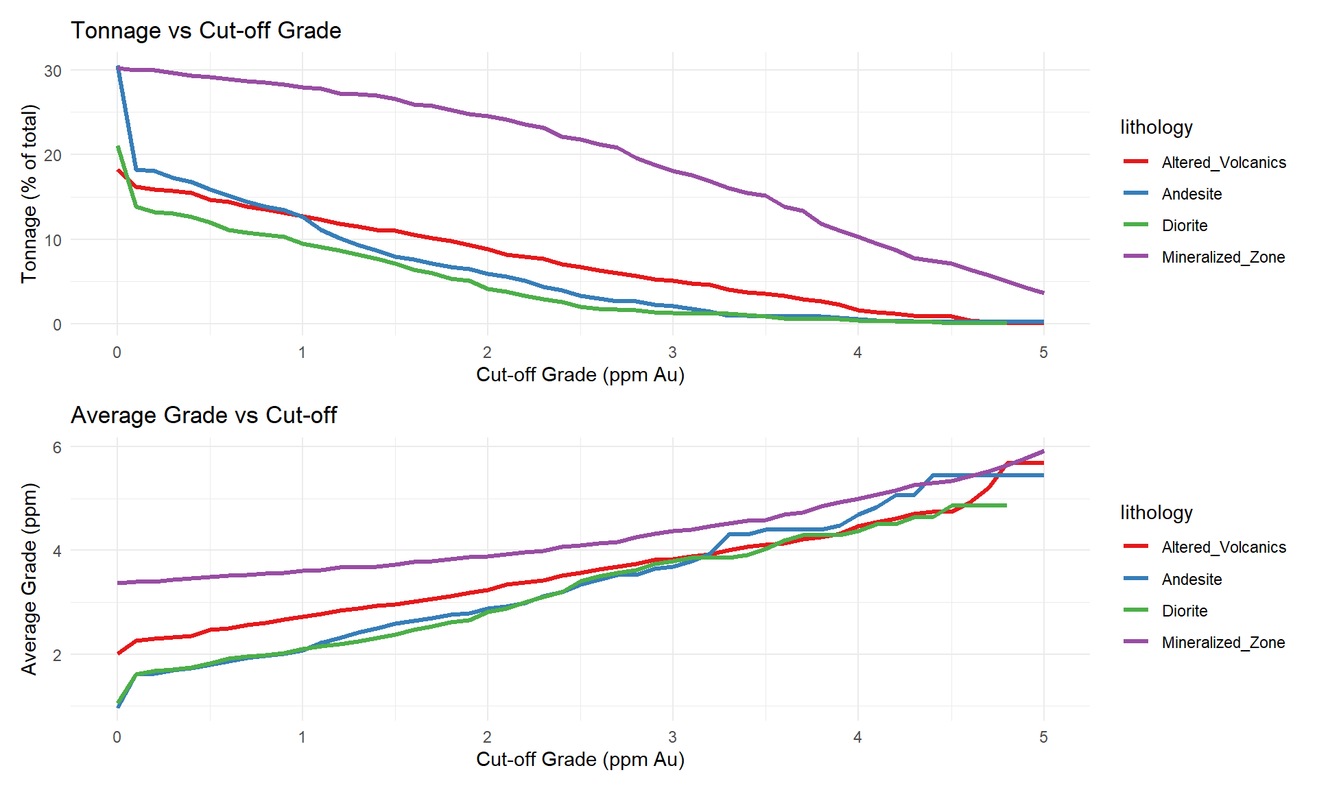
### Grade-Tonnage Curves by Lithology
Understanding the economic potential of each rock type.
```{r}
#| fig-width: 10
#| fig-height: 6
#| warning: false
# Calculate grade-tonnage curves
cutoffs <- seq(0, 5, by = 0.1)

gt_curves <- combined_data %>%
  expand_grid(cutoff = cutoffs) %>%
  filter(au_ppm >= cutoff) %>%
  group_by(lithology, cutoff) %>%
  summarise(
    tonnage_pct = n() / nrow(combined_data) * 100,
    avg_grade = mean(au_ppm, na.rm = TRUE),
    .groups = 'drop'
  )

# Plot tonnage vs cutoff
p_tonnage <- ggplot(gt_curves, aes(x = cutoff, y = tonnage_pct, color = lithology)) +
  geom_line(size = 1.2) +
  scale_color_manual(values = litho_colors) +
  labs(
    title = "Tonnage vs Cut-off Grade",
    x = "Cut-off Grade (ppm Au)",
    y = "Tonnage (% of total)"
  ) +
  theme_minimal() +
  theme(legend.position = "right")

# Plot grade vs cutoff
p_grade <- ggplot(gt_curves, aes(x = cutoff, y = avg_grade, color = lithology)) +
  geom_line(size = 1.2) +
  scale_color_manual(values = litho_colors) +
  labs(
    title = "Average Grade vs Cut-off",
    x = "Cut-off Grade (ppm Au)",
    y = "Average Grade (ppm)"
  ) +
  theme_minimal() +
  theme(legend.position = "right")

p_tonnage / p_grade
```
## Part B: Element Correlation Analysis
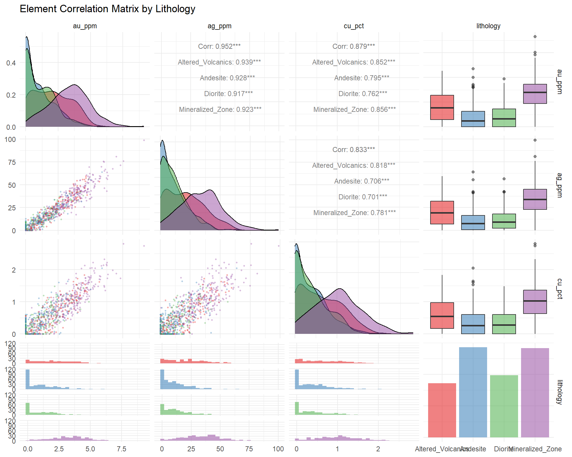
### Bivariate Relationships
Understanding element associations reveals mineralization processes.
```{r}
#| fig-width: 10
#| fig-height: 8
#| warning: false
#| message: false
# Select grade variables for correlation
grade_vars <- c("au_ppm", "ag_ppm", "cu_pct")

# Create scatter plot matrix
suppressWarnings({
  ggpairs(
    combined_data %>% select(all_of(grade_vars), lithology),
    mapping = aes(color = lithology, alpha = 0.5),
    upper = list(continuous = wrap("cor", size = 3)),
    lower = list(continuous = wrap("points", alpha = 0.3, size = 0.5)),
    diag = list(continuous = wrap("densityDiag", alpha = 0.5))
  ) +
    scale_color_manual(values = litho_colors) +
    scale_fill_manual(values = litho_colors) +
    theme_minimal() +
    labs(title = "Element Correlation Matrix by Lithology")
})
```
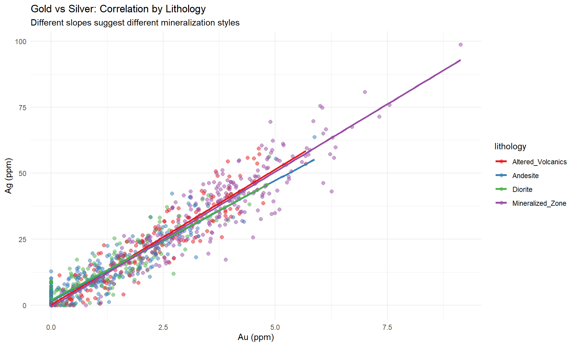
### Regression Analysis: Au vs Ag
```{r}
#| fig-width: 10
#| fig-height: 6
#| warning: false
# Calculate regression by lithology
regression_data <- combined_data %>%
  filter(!is.na(au_ppm) & !is.na(ag_ppm)) %>%
  group_by(lithology) %>%
  filter(n() > 10) %>%
  nest() %>%
  mutate(
    model = purrr::map(data, ~lm(ag_ppm ~ au_ppm, data = .x)),
    r_squared = purrr::map_dbl(model, ~summary(.x)$r.squared),
    slope = purrr::map_dbl(model, ~coef(.x)[2]),
    intercept = purrr::map_dbl(model, ~coef(.x)[1])
  )

# Create scatter plot with regression lines
p_regression <- ggplot(combined_data, aes(x = au_ppm, y = ag_ppm)) +
  geom_point(aes(color = lithology), alpha = 0.5, size = 2) +
  geom_smooth(aes(color = lithology), method = "lm", se = FALSE, size = 1.2) +
  scale_color_manual(values = litho_colors) +
  labs(
    title = "Gold vs Silver: Correlation by Lithology",
    subtitle = "Different slopes suggest different mineralization styles",
    x = "Au (ppm)",
    y = "Ag (ppm)"
  ) +
  theme_minimal() +
  theme(legend.position = "right")

p_regression
```
### Correlation Summary Table
```{r}
regression_summary <- regression_data %>%
  select(lithology, r_squared, slope, intercept) %>%
  arrange(desc(r_squared)) %>%
  mutate(
    equation = paste0("Ag = ", round(slope, 2), " × Au + ", round(intercept, 2)),
    r_squared = round(r_squared, 3)
  ) %>%
  select(lithology, r_squared, equation)

datatable(regression_summary,
          caption = "Table 2: Au-Ag Correlation by Lithology",
          options = list(pageLength = 10, dom = 't')) %>%
  formatStyle(
    'r_squared',
    background = styleColorBar(regression_summary$r_squared, 'lightgreen'),
    backgroundSize = '100% 90%',
    backgroundRepeat = 'no-repeat',
    backgroundPosition = 'center'
  )
```
::: {.callout-tip}
## Geochemical Insights
Strong correlations indicate:
- **Coupled mineralization**: Elements deposited together
- **Common sources**: Shared ore fluids or processes
- **Domain boundaries**: Changes in correlation suggest domain breaks
Weak correlations may indicate:
- **Different mineralization events**: Overprinting
- **Remobilization**: Secondary processes
- **Mixed populations**: Need for further domain subdivision
:::
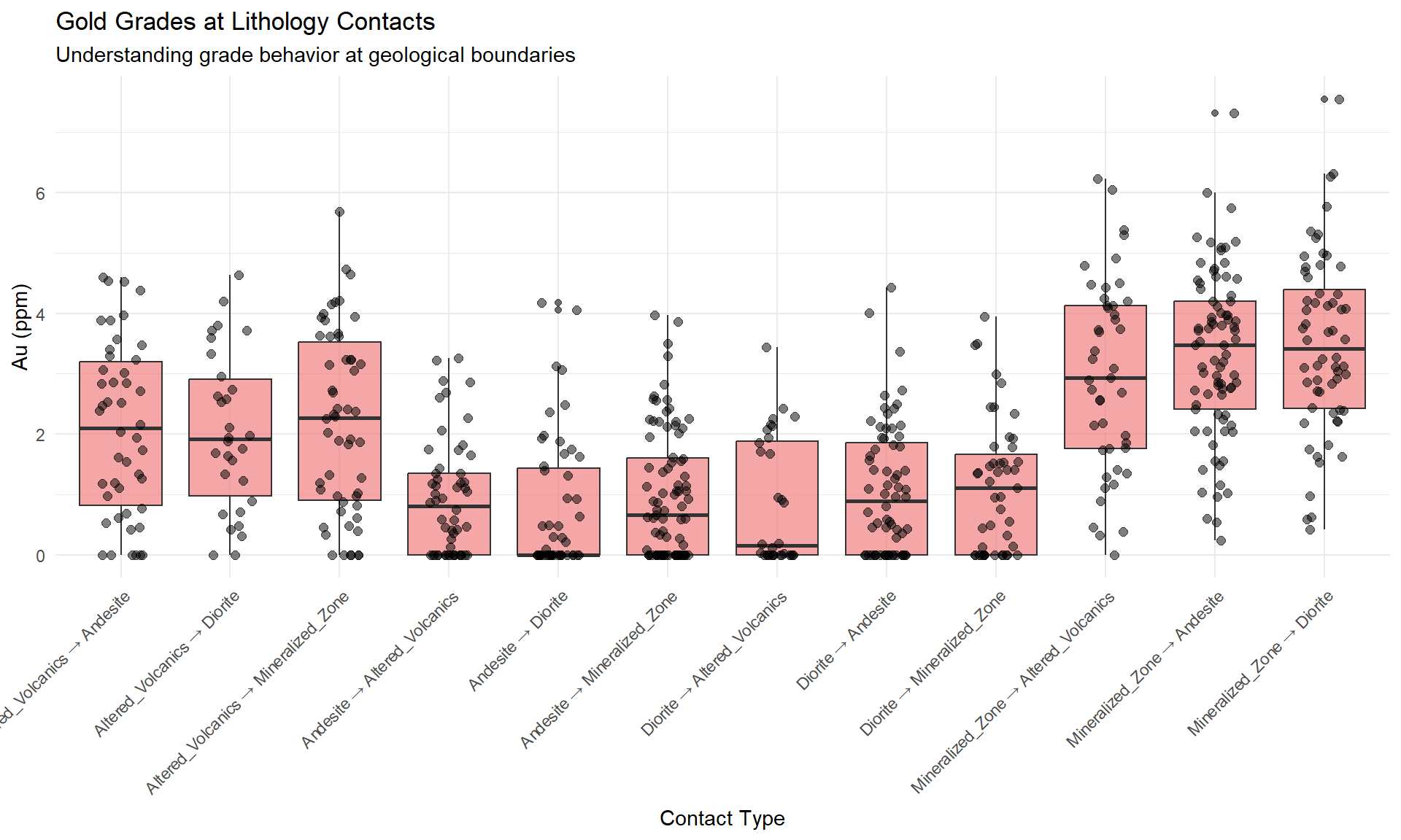
## Part C: Contact Analysis
### Grade Behavior at Geological Boundaries
How does grade change across lithology contacts?
```{r}
#| fig-width: 10
#| fig-height: 6
#| warning: false
# Identify contact zones (simplified approach)
contact_zones <- combined_data %>%
  arrange(hole_id, from) %>%
  group_by(hole_id) %>%
  mutate(
    next_litho = lead(lithology),
    is_contact = lithology != next_litho & !is.na(next_litho),
    contact_type = if_else(is_contact,
                          paste(lithology, "→", next_litho),
                          NA_character_)
  ) %>%
  filter(is_contact) %>%
  ungroup()

# Plot grade at contacts
if(nrow(contact_zones) > 0) {
  p_contacts <- ggplot(contact_zones, aes(x = contact_type, y = au_ppm)) +
    geom_boxplot(fill = "lightcoral", alpha = 0.7) +
    geom_jitter(width = 0.2, alpha = 0.5, size = 2) +
    labs(
      title = "Gold Grades at Lithology Contacts",
      subtitle = "Understanding grade behavior at geological boundaries",
      x = "Contact Type",
      y = "Au (ppm)"
    ) +
    theme_minimal() +
    theme(axis.text.x = element_text(angle = 45, hjust = 1))

  print(p_contacts)
} else {
  cat("No contact zones identified in the dataset.\n")
}
```
::: {.callout-note}
## Contact Zone Interpretation
Sharp grade changes at contacts may indicate:
- **Structural controls**: Faults or shears
- **Alteration halos**: Gradational vs sharp boundaries
- **Domain boundaries**: Where to draw estimation domains
- **Dilution zones**: Material to exclude from ore domains
:::
## Domain Definition Workflow
### Combining All Evidence
Now we synthesize findings from all analyses:
```{r}
#| warning: false
# IMPROVED: More realistic domain classification
# Step 1: Classify each interval
domain_definition <- combined_data %>%
  mutate(
    interval_domain = case_when(
      lithology == "Mineralized_Zone" & au_ppm >= 1.5 ~ "High Grade Ore",
      lithology == "Mineralized_Zone" & au_ppm >= 0.3 ~ "Low Grade Ore",
      lithology == "Altered_Volcanics" & au_ppm >= 0.8 ~ "Altered Ore",
      au_ppm < 0.3 ~ "Waste",
      TRUE ~ "Transitional"
    )
  )

# Step 2: Summarize by hole (dominant domain approach)
hole_summary <- domain_definition %>%
  group_by(hole_id) %>%
  summarise(
    n_intervals = n(),
    avg_au = mean(au_ppm, na.rm = TRUE),
    max_au = max(au_ppm, na.rm = TRUE),
    has_high_grade = any(interval_domain == "High Grade Ore"),
    pct_ore = sum(interval_domain %in% c("High Grade Ore", "Low Grade Ore", "Altered Ore")) / n() * 100,
    .groups = 'drop'
  )

# Step 3: Final hole-level domain classification
hole_domains <- hole_summary %>%
  mutate(
    hole_domain = case_when(
      has_high_grade & avg_au >= 1.0 ~ "High Grade Ore",
      avg_au >= 0.8 ~ "Low Grade Ore",
      avg_au >= 0.5 | pct_ore >= 30 ~ "Altered Ore",
      avg_au >= 0.3 ~ "Transitional",
      TRUE ~ "Waste"
    )
  )

# Summary by domain
domain_summary <- domain_definition %>%
  group_by(interval_domain) %>%
  summarise(
    Intervals = n(),
    `Mean Au` = mean(au_ppm, na.rm = TRUE),
    `Median Au` = median(au_ppm, na.rm = TRUE),
    `Mean Ag` = mean(ag_ppm, na.rm = TRUE),
    `Mean Cu` = mean(cu_pct, na.rm = TRUE),
    .groups = 'drop'
  ) %>%
  arrange(desc(`Mean Au`)) %>%
  mutate(across(where(is.numeric) & !Intervals, ~round(.x, 3)))

datatable(domain_summary,
          caption = "Table 3: Proposed Estimation Domains (Interval-Based)",
          options = list(pageLength = 10, dom = 't'))
# Hole-level summary
hole_domain_summary <- hole_domains %>%
  group_by(hole_domain) %>%
  summarise(
    Holes = n(),
    `Avg Au (ppm)` = mean(avg_au),
    `Max Au (ppm)` = max(max_au),
    .groups = 'drop'
  ) %>%
  arrange(desc(`Avg Au (ppm)`)) %>%
  mutate(across(where(is.numeric) & !Holes, ~round(.x, 3)))

datatable(hole_domain_summary,
          caption = "Table 4: Domain Classification by Drillhole",
          options = list(pageLength = 10, dom = 't'))
```
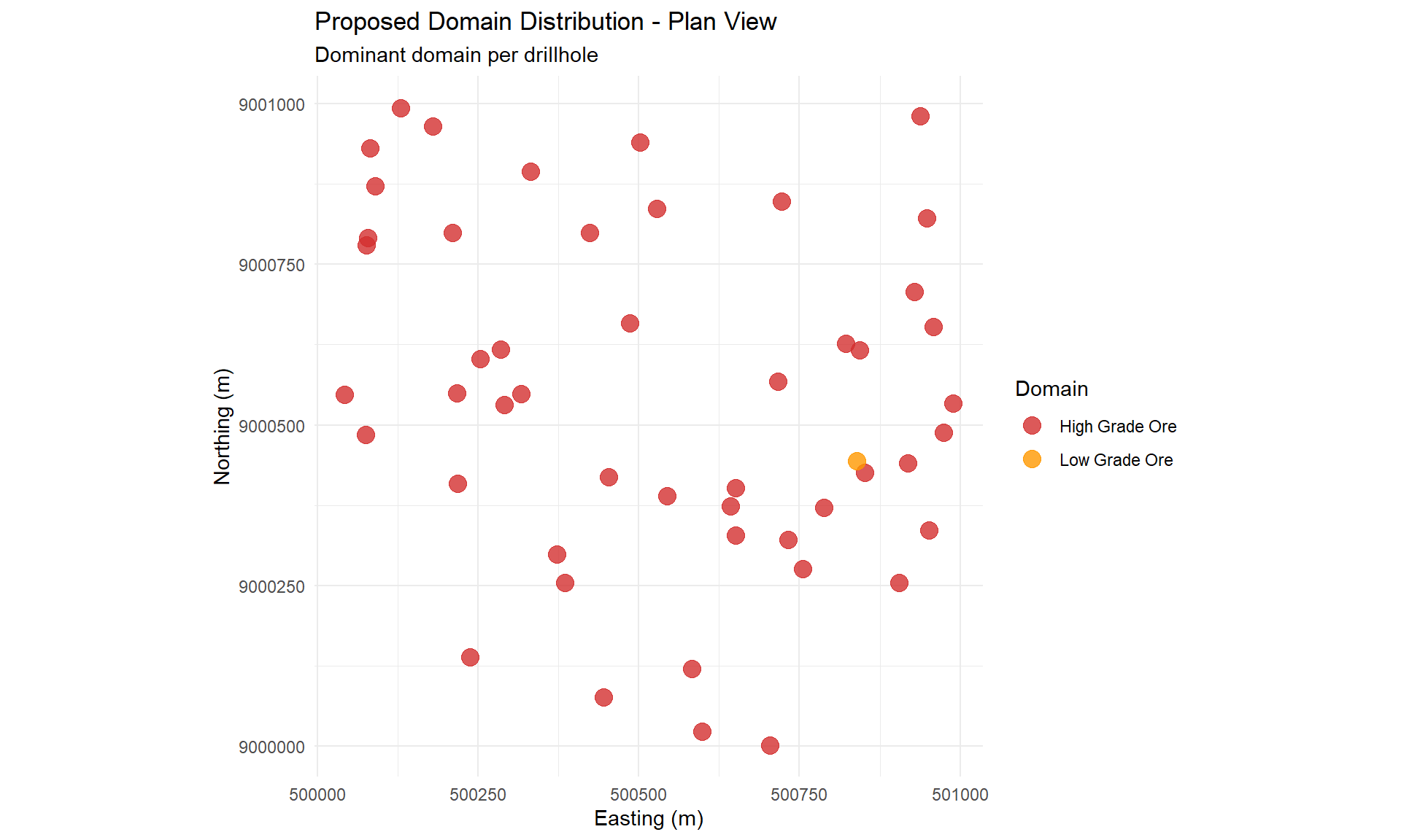
### Domain Spatial Distribution
```{r}
#| fig-width: 10
#| fig-height: 6
#| warning: false
# Create color palette for domains
domain_colors <- c(
  "High Grade Ore" = "#d32f2f",
  "Low Grade Ore" = "#ff9800",
  "Altered Ore" = "#ffd54f",
  "Transitional" = "#9e9e9e",
  "Waste" = "#e0e0e0"
)

# Merge hole domains with collar data
domain_spatial <- hole_domains %>%
  left_join(collar_std, by = "hole_id")

p_domain_map <- ggplot(domain_spatial, aes(x = x, y = y, color = hole_domain)) +
  geom_point(size = 4, alpha = 0.8) +
  scale_color_manual(values = domain_colors) +
  coord_equal() +
  labs(
    title = "Proposed Domain Distribution - Plan View",
    subtitle = "Dominant domain per drillhole",
    x = "Easting (m)",
    y = "Northing (m)",
    color = "Domain"
  ) +
  theme_minimal() +
  theme(legend.position = "right")

p_domain_map
```
## The Birth of Robust Geological Domains
### Before EDA
Without systematic EDA:
- Random data points without geological context
- Mixed populations in estimation
- Unreliable variograms
- Poor mining selectivity
### After EDA: The 4 Pillars Converge
```{mermaid}
flowchart TB
    P1[Pillar 1:<br/>Clean, Validated Data] --> D[Robust<br/>Geological<br/>Domains]
    P2[Pillar 2:<br/>Spatial Understanding] --> D
    P3[Pillar 3:<br/>Statistical Populations] --> D
    P4[Pillar 4:<br/>Geological Controls] --> D

    D --> E1[Reliable Estimation]
    D --> E2[Realistic Mine Plans]
    D --> E3[Confident Classification]

    style D fill:#4caf50,color:#fff
    style P1 fill:#e3f2fd
    style P2 fill:#fff3e0
    style P3 fill:#f3e5f5
    style P4 fill:#e8f5e9
```
### Domain Validation Checklist
::: {.callout-important}
## Defensible Domains Must Have:
✓ **Geological justification**: Rock types, alteration, structure
✓ **Statistical support**: Distinct populations, different variability
✓ **Spatial continuity**: Mappable in 3D space
✓ **Grade differences**: Economically meaningful
✓ **Sample support**: Adequate data density
✓ **Clear boundaries**: Definable contacts
:::
## Summary: From Data to Domains
### What We Accomplished
Through the 4 Pillar EDA framework, we:
1. **Validated data integrity** (Pillar 1)
2. **Understood spatial distribution** (Pillar 2)
3. **Characterized grade populations** (Pillar 3)
4. **Identified geological controls** (Pillar 4)
**Result**: Scientifically defensible estimation domains ready for resource modeling.
### Next Steps in Resource Estimation
With robust domains defined, you can proceed to:
1. **Compositioning**: Regularize sample support within domains
2. **Variography**: Model spatial continuity per domain
3. **Estimation**: Kriging with appropriate search parameters
4. **Classification**: Measured, Indicated, Inferred categories
5. **Validation**: Check estimates against reality
### Key Takeaways
::: {.callout-tip}
## Remember These Principles
1. **EDA is not optional** - It's mandatory for JORC compliance
2. **Data quality = Model reliability** - GIGO always applies
3. **Geology drives domains** - Statistics support, geology defines
4. **Document everything** - Auditors will ask for justification
5. **Use modern tools** - Automate routine tasks, focus on interpretation
:::
## Impact on Business Decisions
Good EDA and domaining directly impact:
- **Resource confidence**: Better classification categories
- **Mine planning**: Realistic extraction sequences
- **Grade control**: Achievable selectivity
- **Investor confidence**: Defensible, auditable reports
- **Project value**: Reduced risk = higher valuations
::: {.callout-important}
## The Foundation of Trust
"In mining, we don't get second chances. The quality of our EDA determines whether we build a mine or lose millions in poor decisions."
**Every successful operation starts with understanding the data.**
:::
## Tools and Resources
### GeoDataViz Application
All analyses demonstrated here are available in GeoDataViz:
- **GitHub**: [github.com/ghoziankarami/GeoDataViz](https://github.com/ghoziankarami/GeoDataViz/)
- **Zenodo**: [doi.org/10.5281/zenodo.17142676](https://doi.org/10.5281/zenodo.17142676)
- **License**: MIT (Open Source)
### Contact
- **Author**: Ghozian Islam Karami
- **Email**: ghoziankarami@gmail.com
- **LinkedIn**: [linkedin.com/in/ghoziankarami](https://linkedin.com/in/ghoziankarami)
---
## Series Complete
You've completed the comprehensive EDA workflow:
- [← Part 1: Foundation & Data Validation](../Data Validation/)
- [← Part 2: Spatial & Statistical Analysis](../Spatial Statistics/)
- **Part 3: Geological Controls & Domain Definition** (You are here)
You now have the tools and knowledge to build **trusted geological models** from raw drilling data.
---
*"Quality data, systematic analysis, geological thinking - the foundation of every successful mine."*